Multi-objective

Throughout this section, we will solve the two-objective problem ZDT1 imported from pymoo.

For more details about the algorithms used, please refer to the Algorithms section.

ZDT1

Consider \(n=30\).

\[\begin{split}\begin{align} \text{min} \; \; & f_1(\boldsymbol{x}) = x_1\\ & f_2(\boldsymbol{x}) = g(\boldsymbol{x}) h(f_1(\boldsymbol{x}), \boldsymbol{x})\\ \text{s.t.} \; \; & g(\boldsymbol{x}) = 1 + \frac{9}{n - 1} \sum_{i=1}^{n}x_i\\ & h(f_1, g) = 1 - \sqrt{ \frac{f_1}{g} }\\ & 0.0 \leq \boldsymbol{x} \leq 1.0 \end{align}\end{split}\]

import matplotlib.pyplot as plt
from pymoo.indicators.igd import IGD
from pymoo.optimize import minimize
from pymoo.problems import get_problem

from pymoode.algorithms import GDE3, NSDE
from pymoode.performance import SpacingIndicator
from pymoode.survival import RankAndCrowding

problem = get_problem('zdt1')
pf = problem.pareto_front()

NGEN = 250
POPSIZE = 100
SEED = 5

GDE3

Let us instantiate a GDE3 algorithm and pass as the default survival operator RankAndCrowding(crowding_func="cd"), which is suitable for problems with two objectives.

gde3 = GDE3(
    pop_size=POPSIZE,
    variant='DE/rand/1/bin',
    CR=0.5,
    F=(0.0, 0.9),
    de_repair='bounce-back',
    survival=RankAndCrowding(crowding_func='cd'),
)

res_gde3 = minimize(
    problem,
    gde3,
    ('n_gen', NGEN),
    seed=SEED,
    save_history=False,
    verbose=False,
)

fig, ax = plt.subplots(figsize=[6, 5], dpi=70)
ax.scatter(pf[:, 0], pf[:, 1], color='navy', label='True Front')
ax.scatter(res_gde3.F[:, 0], res_gde3.F[:, 1], color='firebrick', label='GDE3')
ax.set_ylabel('$f_2$')
ax.set_xlabel('$f_1$')
ax.legend()
fig.tight_layout()
plt.show()

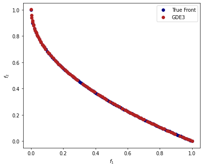
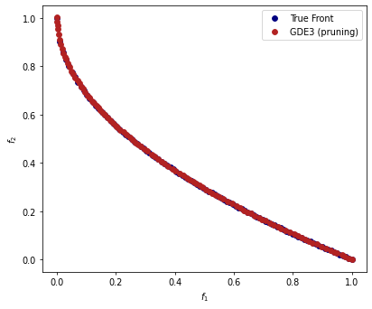
Let us instantiate a GDE3 algorithm and pass as the improved survival operator RankAndCrowding(crowding_func="pcd"), which recursively re-calculates crowding distances as removes individuals from the population. Alternatively, one could have directly imported the GDE3P algorithm.

from pymoode.algorithms import GDE3P

gde3p = GDE3(
    pop_size=POPSIZE,
    variant='DE/rand/1/bin',
    CR=0.5,
    F=(0.0, 0.9),
    de_repair='bounce-back',
    survival=RankAndCrowding(crowding_func='pcd'),
)

res_gde3p = minimize(
    problem,
    gde3p,
    ('n_gen', NGEN),
    seed=SEED,
    save_history=False,
    verbose=False,
)

fig, ax = plt.subplots(figsize=[6, 5], dpi=70)
ax.scatter(pf[:, 0], pf[:, 1], color='navy', label='True Front')
ax.scatter(
    res_gde3p.F[:, 0],
    res_gde3p.F[:, 1],
    color='firebrick',
    label='GDE3 (pruning)',
)
ax.set_ylabel('$f_2$')
ax.set_xlabel('$f_1$')
ax.legend()
fig.tight_layout()
plt.show()

NSDE

Now let us adopt the NSDE algorithm. It is very similar to GDE3, however, adopting a pure \((\mu + \lambda)\) survival strategy, which might lead to premature convergence in some problems of the ZDT test suite.

nsde = NSDE(
    pop_size=POPSIZE,
    variant='DE/rand/1/bin',
    CR=0.5,
    F=(0.0, 0.9),
    de_repair='bounce-back',
    survival=RankAndCrowding(crowding_func='pcd'),
)

res_nsde = minimize(
    problem,
    nsde,
    ('n_gen', NGEN),
    seed=SEED,
    save_history=False,
    verbose=False,
)

fig, ax = plt.subplots(figsize=[6, 5], dpi=70)
ax.scatter(pf[:, 0], pf[:, 1], color='navy', label='True Front')
ax.scatter(res_nsde.F[:, 0], res_nsde.F[:, 1], color='firebrick', label='NSDE')
ax.set_ylabel('$f_2$')
ax.set_xlabel('$f_1$')
ax.legend()
fig.tight_layout()
plt.show()

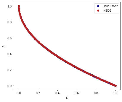
But it worked very well in this example.

Spacing

The spacing indicator is a quantitative metric of how good is the distribution of elements in the pareto front. It is described in more detail in the complete tutorial. One can also refer to [12] for more details.

sp = SpacingIndicator(pf=problem.pareto_front(), zero_to_one=True)

The lesser the spacing, the more even the distribution of elements

print('Spacing of GDE3 with normal crowding distances: ', sp.do(res_gde3.F))
print(
    'Spacing of GDE3 with pruning nds crowding distances: ', sp.do(res_gde3p.F)
)
print(
    'Spacing of NSDE with pruning nds crowding distances: ', sp.do(res_nsde.F)
)

Spacing of GDE3 with normal crowding distances:  0.00671798902242222
Spacing of GDE3 with pruning nds crowding distances:  0.0026884699308083585
Spacing of NSDE with pruning nds crowding distances:  0.002587892035294526

igd = IGD(pf=problem.pareto_front(), zero_to_one=True)

print('IGD of GDE3 with normal crowding distances: ', igd.do(res_gde3.F))
print('IGD of GDE3 with pruning nds crowding distances: ', igd.do(res_gde3p.F))
print('IGD of NSDE with pruning nds crowding distances: ', igd.do(res_nsde.F))

IGD of GDE3 with normal crowding distances:  0.004552975587711302
IGD of GDE3 with pruning nds crowding distances:  0.0038818313760975985
IGD of NSDE with pruning nds crowding distances:  0.0039248610073845105